

Introduction
Imagine you are conducting a study to determine whether a new drug effectively reduces blood pressure. You administer the drug to a group of patients and compare their results to a control group receiving a placebo. You analyze the data and conclude that the new drug significantly reduces blood pressure when, in reality, it does not. This incorrect rejection of the null hypothesis (that the drug has no effect) is a Type I error. On the other hand, suppose the drug actually does reduce blood pressure, but your study fails to detect this effect due to insufficient sample size or variability in the data. As a result, you conclude that the drug is ineffective, which is a failure to reject a false null hypothesis—a Type II error.
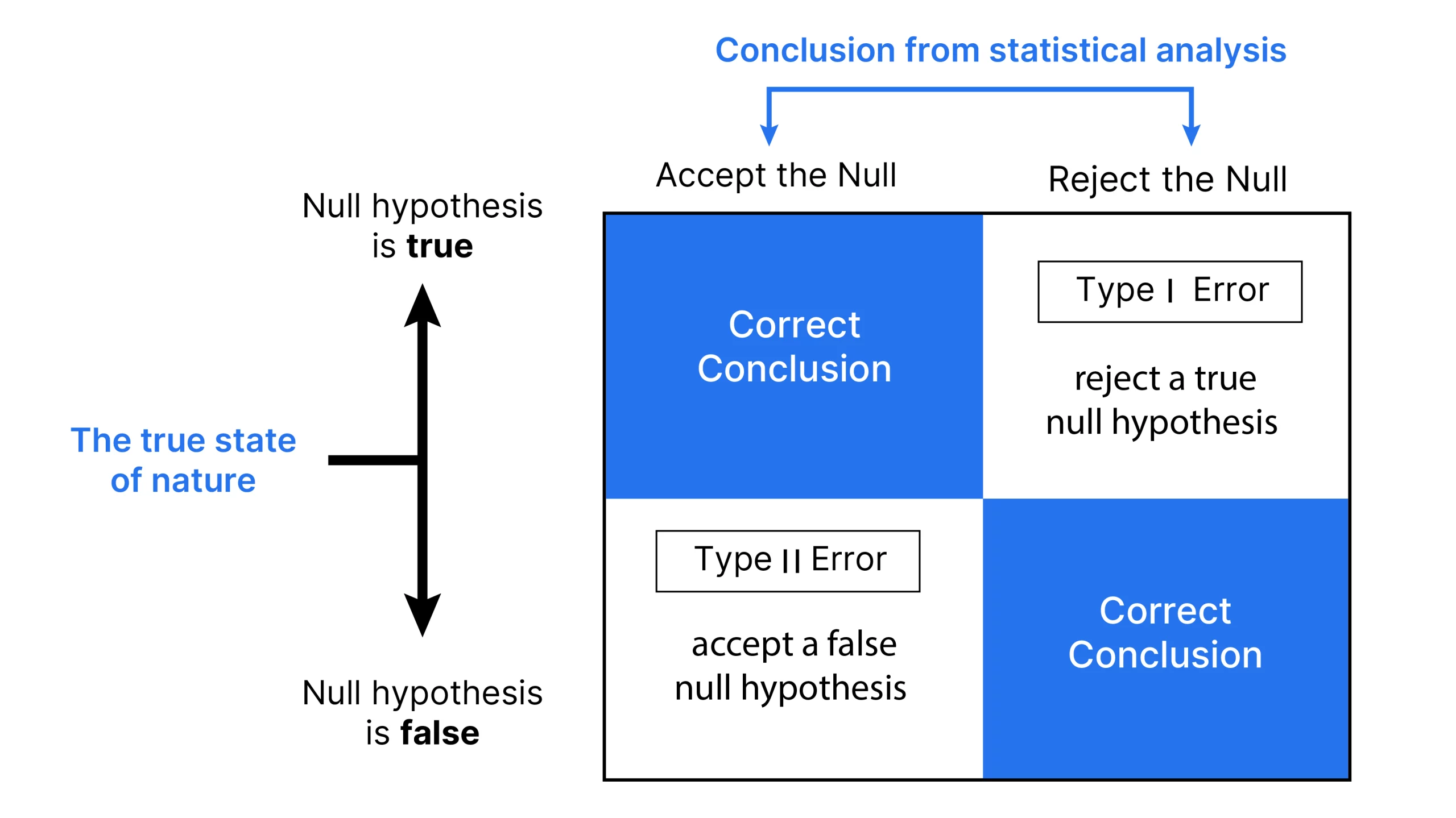
These scenarios highlight the importance of understanding Type I and Type II errors in statistical testing. Type I errors, also known as false positives, occur when we mistakenly reject a true null hypothesis. Type II errors, or false negatives, happen when we fail to reject a false null hypothesis. Much of statistical theory revolves around minimizing these errors, though completely eliminating both is statistically impossible. By understanding these concepts, we can make more informed decisions in various fields, from medical testing to quality control in manufacturing.

Overview
- Type I and Type II errors represent false positives and false negatives in hypothesis testing.
- Hypothesis testing involves formulating null and alternative hypotheses, choosing a significance level, calculating test statistics, and making decisions based on critical values.
- Type I errors occur when a true null hypothesis is mistakenly rejected, leading to unnecessary interventions.
- Type II errors happen when a false null hypothesis is not rejected, causing missed diagnoses or overlooked effects.
- Balancing Type I and Type II errors involves trade-offs in significance levels, sample sizes, and test power to minimize both errors effectively.
The Basics of Hypothesis Testing
Hypothesis testing is a method used to decide whether there is enough evidence to reject a null hypothesis (H₀) in favor of an alternative hypothesis (H₁). The process involves:
- Formulating Hypotheses
- No effect or no difference: No effect or no difference.
- Alternative Hypothesis (H₁): An effect or a difference exists.
- Choosing a Significance Level (α): The probability threshold for rejecting H₀, typically set at 0.05, 0.01, or 0.10.
- Calculating the Test Statistic: A value derived from sample data used to compare against a critical value.
- Making a Decision: If the test statistic exceeds the crucial value, reject H₀; otherwise, do not reject H₀.
Also read: End-to-End Statistics for Data Science
Type 1 Error( False Positive)
A Type I error occurs when an experiment’s null hypothesis(H0) is true but mistakenly rejected (the Graph is mentioned below).
This error represents identifying something that is not actually present, similar to a false positive. This can be explained in simple terms with an example: In a medical test for a disease, a Type I error would mean the test indicates a patient has the disease when they do not, essentially raising a false alarm. In this case, the null hypothesis(H0) would state: The patient does not have disease.
The likelihood of committing a Type I error is called the significance level or rate level. It’s denoted by the Greek letter α (alpha) and is known as the alpha level. Typically, this chance or probability is set at 0.05 or 5%. This way, researchers are usually inclined to accept a 5% chance of incorrectly rejecting the null hypothesis when it is sincerely actual.
Type I errors can lead to unnecessary treatments or interventions, causing stress and potential harm to individuals.
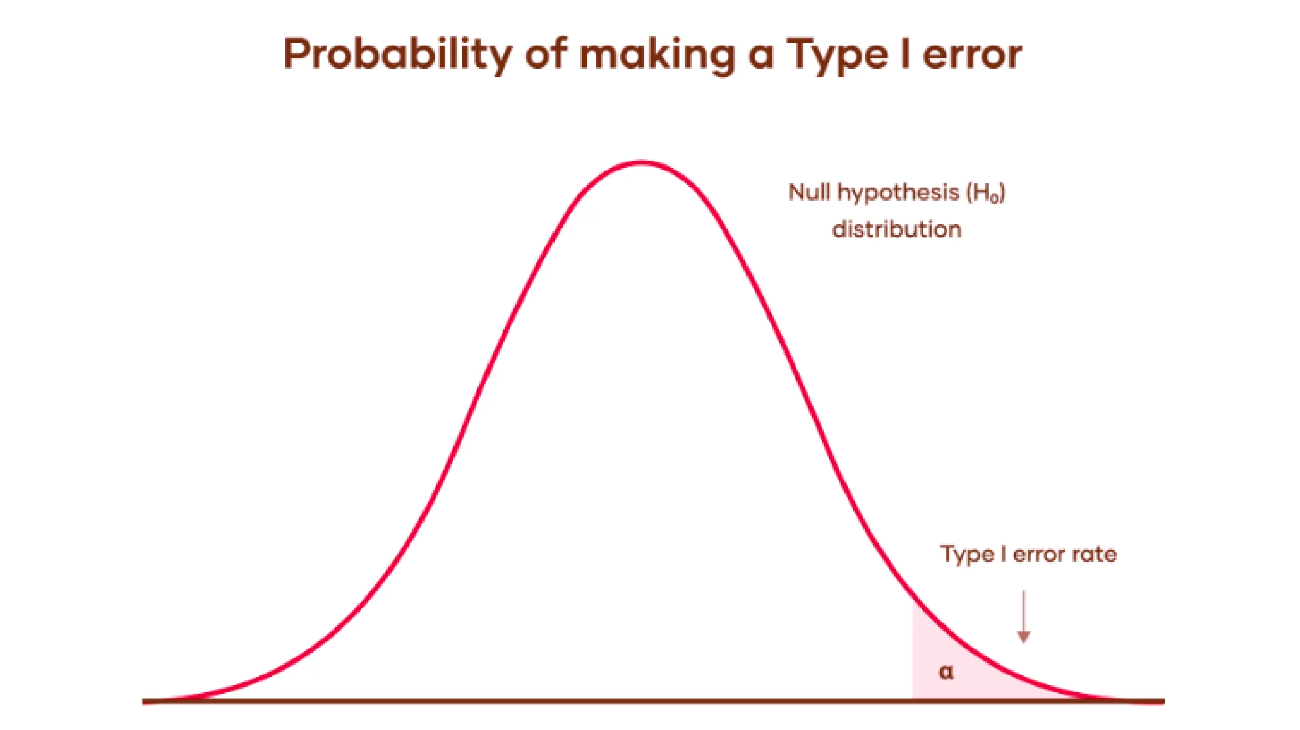
Let’s understand this with Graph:
- Null Hypothesis Distribution: The bell curve shows the range of possible outcomes if the null hypothesis is true. This means the results are due to random chance without any actual effect or difference.
- Type I Error Rate: The shaded area under the curve’s tail represents the significance level, α. It is the probability of rejecting the null hypothesis when it is actually true. Which results in a Type I error (false positive).
Type 2 Error ( False Negative)
A Type II error happens when a valid alternative hypothesis goes unrecognized. In simpler terms, it’s like failing to spot a bear that’s actually there, thus not raising an alarm when one is needed. In this scenario, the null hypothesis (H0) still states, “There is no bear.” The investigator commits a Type II error if a bear is present but undetected.
The key difficulty isn’t always whether the disease exists but whether it is effectively diagnosed. The error can arise in two ways: either by failing to discover the disease when it’s present or by claiming to discover the disease when it is not present.
The probability of Type II error is denoted by the Greek letter β (beta). This value is related to a test’s statistical power, which is calculated as 1 minus β (1−β).
Type II errors can result in missed diagnoses or overlooked effects, leading to inadequate treatment or interventions.
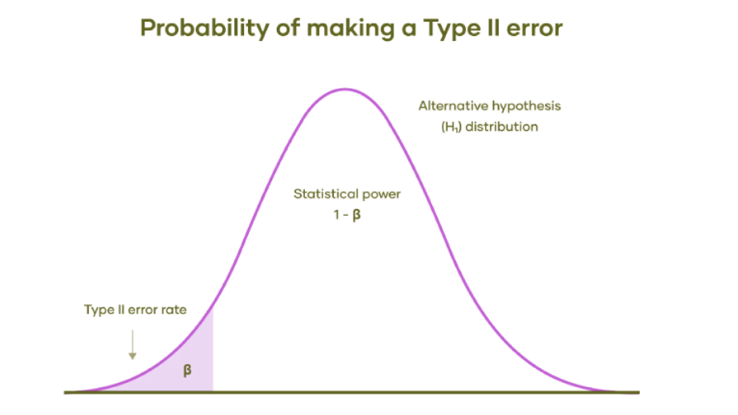
Let’s understand this with Graph:
- Alternative Hypothesis Distribution: The bell curve represents the range of possible outcomes if the alternative hypothesis is true. This means there is an actual effect or difference, contrary to the null hypothesis.
- Type II Error Rate (β): The shaded area under the left tail of the distribution represents the probability of a Type II error.
- Statistical Power (1 – β): The unshaded area under the curve to the right of the shaded area represents the test’s statistical power. Statistical power is the probability of correctly rejecting the null hypothesis when the alternative hypothesis is true. Higher power means a lower chance of making a Type II error.
Also read: Learn all About Hypothesis Testing!
Comparison of Type I and Type II Errors
Here is the detailed comparison:
| Aspect | Type I Error | Type II Error |
|---|---|---|
| Definition and Terminology | Rejecting a true null hypothesis (false positive) | Accepting a false null hypothesis (false negative) |
| Symbolic Representation | α (alpha) | β (beta) |
| Probability and Significance | Equal to the level of significance set for the test | Calculated as 1 minus the power of the test (1 – power) |
| Error Reduction Strategies | Decrease the level of significance (increases Type II errors) | Increase the level of significance (raises Type I errors) |
| Causal Factors | Chance or luck | Smaller sample sizes or less powerful statistical tests |
| Analogies | “False hit” in a detection system | “Miss” in a detection system |
| Hypothesis Association | Incorrectly rejecting the null hypothesis | Failing to reject a false null hypothesis |
| Occurrence Conditions | Occurs when acceptance levels are too lenient | Occurs when acceptance criteria are overly stringent |
| Implications | Prioritized in fields where avoiding false positives is crucial (e.g., clinical testing) | Prioritized in fields where avoiding false negatives is crucial (e.g., screening for severe diseases) |
Also read: Hypothesis Testing Made Easy for Data Science Beginners
Trade-off Between Type I and Type II Errors
There is mostly a trade-off among Type I and Type II errors. Reducing the likelihood of one type of error generally increases the opportunity for the opposite.
- Significance Level (α): Lowering α reduces the chance of a Type I error but increases the risk of a Type II error. Increasing α has the opposite effect.
- Sample Size: Increasing the sample size can reduce both Type I and Type II errors, as larger samples provide more accurate estimates.
- Test Power: Enhancing the test’s power by increasing the sample size or using more sensitive tests can reduce the probability of Type II errors.
Conclusion
Type I and Type II errors are fundamental ideas in statistics and research techniques. By knowing the difference between these errors and their implications, we can interpret research findings better, conduct more powerful research, and make more informed decisions in diverse fields. Remember, the goal isn’t to eliminate errors (which is impossible) but to manage them successfully based on the particular context and potential outcomes.
Frequently Asked Questions
Ans. It’s challenging to eliminate both types of errors because reducing one often increases the other. However, by increasing the sample size and carefully designing the study, researchers can decrease both errors to applicable levels.
Ans. Here are the common misconceptions about Type I and Type II errors:
Misconception: A lower α always means a better test.
Reality: While a lower α reduces Type I errors, it can increase Type II errors, leading to missed detections of true effects.
Misconception: Large sample sizes eliminate the need to worry about these errors.
Reality: Large sample sizes reduce errors but do not eliminate them. Good study design is still essential.
Misconception: A significant result (p-value < α) means the null hypothesis is false.
Reality: A significant result suggests evidence against H₀, but it does not prove H₀ is false. Other factors like study design and context must be considered.
Ans. Increasing the power of your test makes it more likely to detect a true effect. You can do this by:
A. Increasing your sample size.
B. Using more precise measurements.
C. Reducing variability in your data.
D. Increasing the effect size, if possible.
Ans. Pilot studies help you estimate the parameters needed to design a larger, more definitive study. They provide initial data on effect sizes and variability, which inform your sample size calculations and help balance Type I and Type II errors in the main study.